The model begins scoring its own rollout.

A recently published study proposes a highly practical idea: have a diffusion model first roll out forward in time, then switch direction and retrace its path. If the model cannot return to its starting point, the round-trip discrepancy can serve as a proxy metric for long-horizon generation error.

The work is titled Round-Trip Consistency, with paper ID arXiv:2608.00675, and its code and data-generation pipeline have been open-sourced. Rather than focusing on single-image generation, it targets dynamic systems such as video, turbulent flow fields, and digital twins: the model predicts the next state at each step, then feeds its own output back into itself. As the number of steps increases, small errors are repeatedly amplified. Yet during deployment, future ground truth is usually unavailable for comparison, making it impossible to know when the model has begun to “drift off course.”

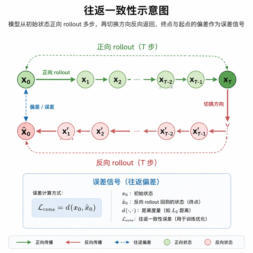
The research team’s solution is to train a conditional latent diffusion model with a direction indicator, allowing the same set of parameters to both predict the future and infer the past from a future state. The model advances forward for several steps and then moves backward for the same number of steps. The distance between the final state and the initial state is called the round-trip consistency error.

What makes this especially noteworthy is not that “diffusion models can run backward,” but that the method turns the model’s otherwise unused reverse capability into a warning light that requires no measurement data.

The Biggest Problem With Long-Horizon Models Is That They Do Not Know When They Are Wrong

First, let us distinguish between two concepts that are often conflated.

A diffusion model may generate a state internally through multiple denoising steps, but when used for dynamic prediction, its outer loop may still be an autoregressive rollout:

1. Given the current state x₀, generate the next state x₁;
2. Treat the generated x₁ as the true input and continue generating x₂;
3. Repeat the process to obtain x₃, x₄, and so on.

Therefore, even if the single-step predictor is a latent diffusion or flow model, the overall temporal rollout still suffers from the classic problem of error accumulation. During training, the model usually sees real historical states; during deployment, however, an increasing proportion of its inputs are its own generated outputs. This distribution mismatch grows with the rollout length.

On facial-video datasets such as CelebV-HQ, the initial issue may be only a slight deviation in the corners of the mouth or the gaze. After dozens of frames, however, it may turn into identity drift, texture flickering, or discontinuous motion. In physical settings such as turbulence, local phase errors can alter the subsequent evolution path, ultimately producing a sequence that looks visually smooth and has realistic-looking statistics, even though its specific state has long since diverged from the true trajectory.

The problem is that online simulation is precisely where ground truth is unavailable. Otherwise, there would be no need for the model to make predictions.

Common remedies include model ensembles, uncertainty networks, physics residuals, reserved validation sensors, or separately trained error predictors. These approaches respectively require multi-model inference, error labels, governing equations, or additional measurements. In real-world deployments, any of these requirements may be expensive—or may not be available at all.

One Model, One Direction Switch: Go Out, Then Come Back

The model in this work can be simplified as a conditional transition operator:

• It takes the current latent state as input;
• It takes the time interval or related conditions as input;
• It also takes a direction indicator d, where d=+1 means predicting toward the future and d=-1 means inferring backward toward the past;
• It outputs the adjacent state in the specified direction.

Suppose the model runs forward for K steps from the initial state x₀, producing x̂K. It then flips the direction indicator and runs backward for K steps from x̂K, producing the reconstructed starting point x̃₀. The round-trip error can be expressed abstractly as:

R_K = D(x₀, x̃₀)

Here, D may be the mean squared error in state space, a latent-space distance, a perceptual distance, or some task-specific metric. The error we actually want to know—but cannot observe during deployment—is:

E_K = D(xK, x̂K)

The central experimental question is: Can R_K predict E_K?

According to the results reported by the authors, the round-trip discrepancy serves as an effective proxy for the true rollout error in tests involving facial videos, turbulence, and other domains. In other words, the less reliable the forward prediction is, the more difficult it usually is for the model to return to its starting point in the reverse direction.

The inference logic is straightforward. The pseudocode is roughly as follows:

state = start
for i in 1..K:
    state = model(state, direction=forward)

forward_result = state

for i in 1..K:
    state = model(state, direction=backward)

round_trip_score = distance(state, start)

The entire process requires no future ground truth, no governing equations, and no separately trained error classifier. The cost is one additional reverse rollout of equal length: if the original forward simulation requires K steps, the new procedure requires approximately 2K steps in total.

Therefore, “one additional rollout” should not be interpreted as free. What it eliminates is the need for model ensembles and external supervision—not inference compute. For digital-twin simulations running on a minute-level timescale, this trade-off may be highly worthwhile. For video-streaming services requiring millisecond response times, whether to enable it must be decided according to the level of risk.

Why One Shared Model May Outperform Two Specialists

The study also reports an easily overlooked finding: using one network with shared parameters and a direction indicator to learn both forward and backward transitions not only avoids a significant loss in one-way performance, but actually outperforms separately trained forward and backward specialists in both directions.

This can be viewed as a form of structured multitask learning.

Forward data tells the model “where a state will go,” while backward data forces it to understand “where the current state may have come from.” The two tasks share the same latent space and feature extractor, effectively imposing stronger temporal constraints on the dynamic representation. The model cannot merely memorize how to extrapolate local textures; it must also learn which features remain relatively stable across temporal transitions.

This benefit does not mean that bidirectional training is truly cost-free. A single training step may need to process data in both directions, and the data pipeline and condition encoding also become more complex. However, if a shared model can replace two specialist models while maintaining a similar parameter count, it can indeed reduce the costs of deployment storage, model maintenance, and consistency across bidirectional inference.

More importantly, only with a shared model does the round-trip error resemble an interpretable “self-check signal.” If the forward and backward passes are handled by two entirely independent models, the final discrepancy mixes the errors of both models, making it difficult to determine whether an alert was caused by distortion in the forward trajectory or simply by a weak backward specialist.

The Signal Is Useful, but It Should Not Be Called Confidence

The most appealing narrative around round-trip consistency is that “the model knows when it is wrong.” Strictly speaking, that claim goes too far.

The method measures the extent to which the loop fails to close. It is not inherently equivalent to confidence in a probabilistic sense, nor is it guaranteed to correspond monotonically to every type of task error. At least four blind spots require caution.

1. The Forward and Backward Models May Make the Same Mistake Together

If the model learns an incorrect but self-consistent dynamic path, it may move forward along the wrong trajectory and still return to the starting point by following that same incorrect trajectory in reverse. In this case, the round-trip error is small even though the predicted future state may be far from the truth.

This is similar to validating primary and replica databases: if two copies are perfectly consistent, that only proves they match each other—not that the data itself is correct.

2. The Real System May Not Be Reversible

Dissipative systems, many-to-one mappings, collision occlusions, and dynamic processes involving unobserved variables may not have a unique reverse trajectory. For example, once an object leaves the frame in a video, later frames alone cannot recover all of its earlier details. Fine-scale information in turbulent flow may also be lost rapidly.

In such cases, the backward model learns a “possible past” in terms of a conditional distribution rather than a strict inverse function. The round-trip error will therefore reflect both forward-prediction failure and uncertainty arising from the inherent irreversibility of the problem.

3. Diffusion Sampling Is Stochastic

When both the forward and backward processes use stochastic sampling, the round-trip distance from a single run may be significantly affected by sampling noise. In practice, engineers may need to fix random seeds, use a deterministic sampler, or perform a small number of repeated estimates and calibrate the resulting score. Otherwise, the same input may produce highly variable self-check results.

However, once repeated sampling is introduced, the computational cost begins to approach that of an ensemble. Balancing stability and cost is therefore an unavoidable deployment challenge.

4. The Distance Function Determines What the Method Cares About

Pixel-level error is highly sensitive to small displacements, yet it may fail to detect severe errors involving identity, physical conservation laws, or semantics. Conversely, an overly abstract latent-space distance may overlook local anomalies.

Video tasks may benefit from combining pixel values, optical flow, and perceptual features. Physical-field tasks are better suited to incorporating spectra, energy distributions, or task-specific statistics. The fact that the method does not require governing equations does not mean that engineering implementations should reject all domain-specific metrics.

The Most Suitable Practical Uses: Alerts, Routing, and Dynamic Truncation

At this stage, round-trip consistency is better suited as a risk score than as an error-correction algorithm. It can tell the system that “this segment of the rollout is not very trustworthy,” but it cannot automatically provide the correct trajectory.

Several realistic applications include:

• Dynamically determining prediction length: As the round-trip score rises, shorten the open-loop rollout and request a new observation earlier to re-anchor the state.
• Triggering high-cost models: Use a lightweight model in low-risk intervals, then switch to a larger model, model ensemble, or numerical solver in high-risk intervals.
• Filtering generated results: Rank candidate trajectories produced from multiple random seeds and prioritize samples with better round-trip consistency.
• Detecting out-of-distribution inputs: If certain types of initial conditions repeatedly fail to close the loop, add them to an active-learning queue and collect more training data.
• Monitoring model degradation online: Even without future labels, track whether the long-term distribution of round-trip scores is drifting.

The most promising option for developers to explore is a dynamic horizon. Many systems habitually predict a fixed 100 steps, but the predictable duration varies across initial states. Stable segments may remain safe for a long time, while strongly nonlinear segments may become distorted after only a dozen steps. The round-trip signal gives the model an opportunity to adjust the prediction length on a per-sample basis.

A simple deployment strategy could be written as follows:

if round_trip_score < low_threshold:
    accept rollout
elif round_trip_score < high_threshold:
    shorten horizon and request observation sooner
else:
    reject rollout or switch to expensive fallback

The thresholds still need to be calibrated on offline data with ground truth. “Unsupervised validation” means that testing does not rely on future measurements from the current trajectory; it does not mean that the entire training and deployment pipeline requires no labels or validation set whatsoever.

What It Adds to Long-Horizon Generation Is a Dashboard, Not a Seat Belt

The value of this study lies in turning temporal reversibility from a modeling capability into a deployment-time monitoring capability. Compared with training a separate error predictor, it does not require purpose-built labels indicating “how wrong the model is.” Compared with model ensembles, it maintains only one shared network. Compared with physics residuals, it does not require the system to have usable explicit equations.

Moreover, the idea is not limited to diffusion models. As long as a dynamic generator can learn conditional transitions in both forward and backward directions, a similar cycle-consistency signal can in principle be constructed. Diffusion models simply happen to be good at representing multimodal conditional distributions, making them a natural fit for scenarios in which “one future may correspond to multiple possible pasts.”

However, the method is still some distance from being a general-purpose reliability solution. Rather than focusing on how impressive its correlation looks on a particular dataset, attention should currently be directed toward three engineering questions:

1. After changing the rollout length, sampler, or resolution, does the score remain calibratable?
2. In irreversible, strongly dissipative, and out-of-distribution scenarios, will there be dangerous samples with low scores but high true errors?
3. Can the roughly twofold inference cost be reduced through dynamic spot checks, low-frequency self-checks, or coarse-grained latent-space replay?

Our assessment is that Round-Trip Consistency is a diagnostic metric worth adding to long-horizon generation systems, but it should not yet be presented as evidence that models possess reliable self-awareness. It is more like a warning light on a car’s dashboard: it cannot repair the engine for you, but in the absence of external diagnostic equipment, it can warn you to stop pressing the accelerator.

For video generation, this may mean stopping a long video before identity drift becomes severe. For digital twins, it may mean detecting that a trajectory is no longer trustworthy while the simulation still appears smooth. The ability to determine whether a model is drifting off course when no ground truth is available may be closer to the missing piece required for bringing long-horizon models into production than another marginal improvement in single-step generation metrics.

References

• Reddit: Discussion of the Round-Trip Consistency study: The authors’ introduction to the research motivation, methodology, and main conclusions, along with community discussion.
• GitHub: round-trip-consistency: The project’s open-source repository, containing code for data generation, model training, and analysis.
• Zhihu: An Introduction to the LLaDA Diffusion Language Model: Supplementary material for understanding the bidirectional modeling capabilities of diffusion models; its text-generation setting differs from the dynamic-system rollouts discussed in this article.